Introduction

In the previous blog post, we wrapped up our exploration of the simple-ctx example, which runs graph computations in context mode. As mentioned earlier, this mode is not the best practice for using GGML, as it doesn’t support device backends like CUDA and Metal. In this blog post, we will shift our focus to the simple-backend example, which demonstrates GGML’s complete workflow under backend mode.

Note: This blog series is based on commit 475e012.

Initializing the Backend

Before diving into the code, make sure to update your launch.json to set the debug target to simple-backend. This example overlaps with much of the execution flow from simple-ctx, so here, I will focus on the mechanisms that are new to us.

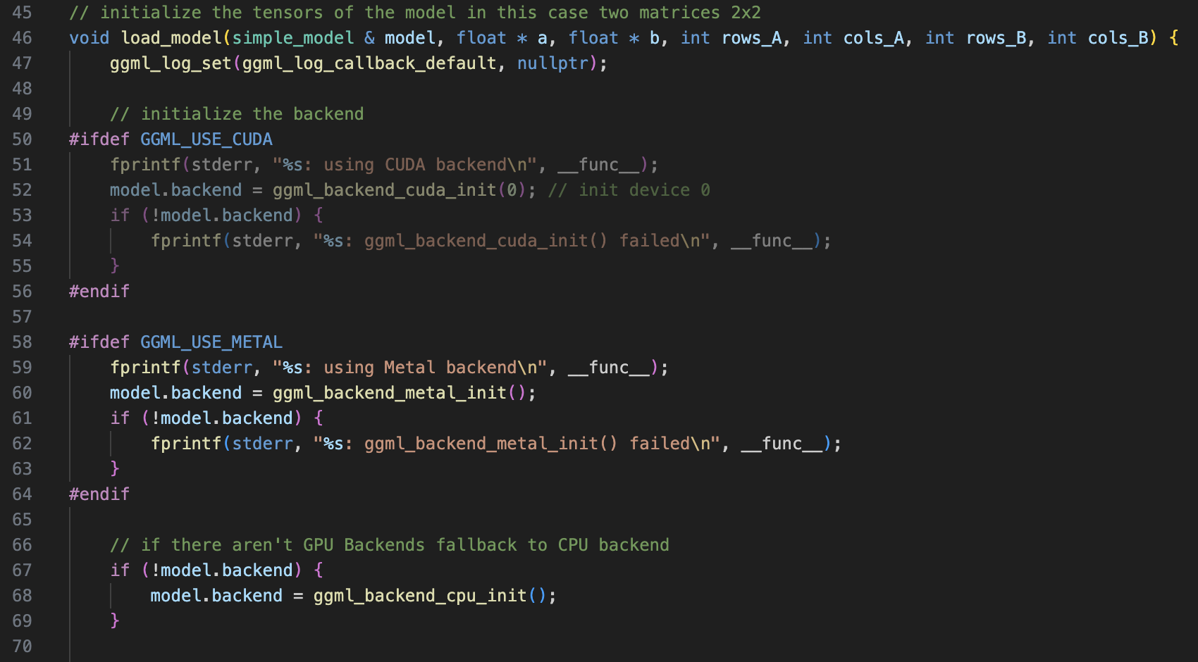
Let’s start by looking at the load_model function. It’s easy to see why this example is called simple-backend: before constructing any in-memory objects like the ggml_context, it first initializes a computing backend. If you don’t have CUDA or Metal backends, don’t worry—this doesn’t affect the example. In fact, all backends can be invoked through a unified interface, so you won’t need to worry about the implementation details for each backend.

Note: In this example, backend selection is straightforward and only three backends (cpu, CUDA and Metal) could be utilized. In future posts we’ll explore how GGML uses a backend registry to manage all available backends.

GGML Backend Classes and Their Relationships

In this section, rather than delving into the specifics of each backend implementation, such as what’s happening inside ggml_backend_cuda_init or ggml_backend_metal_init, I’ll focus on the general structure of GGML backends and how they can be interacted with.

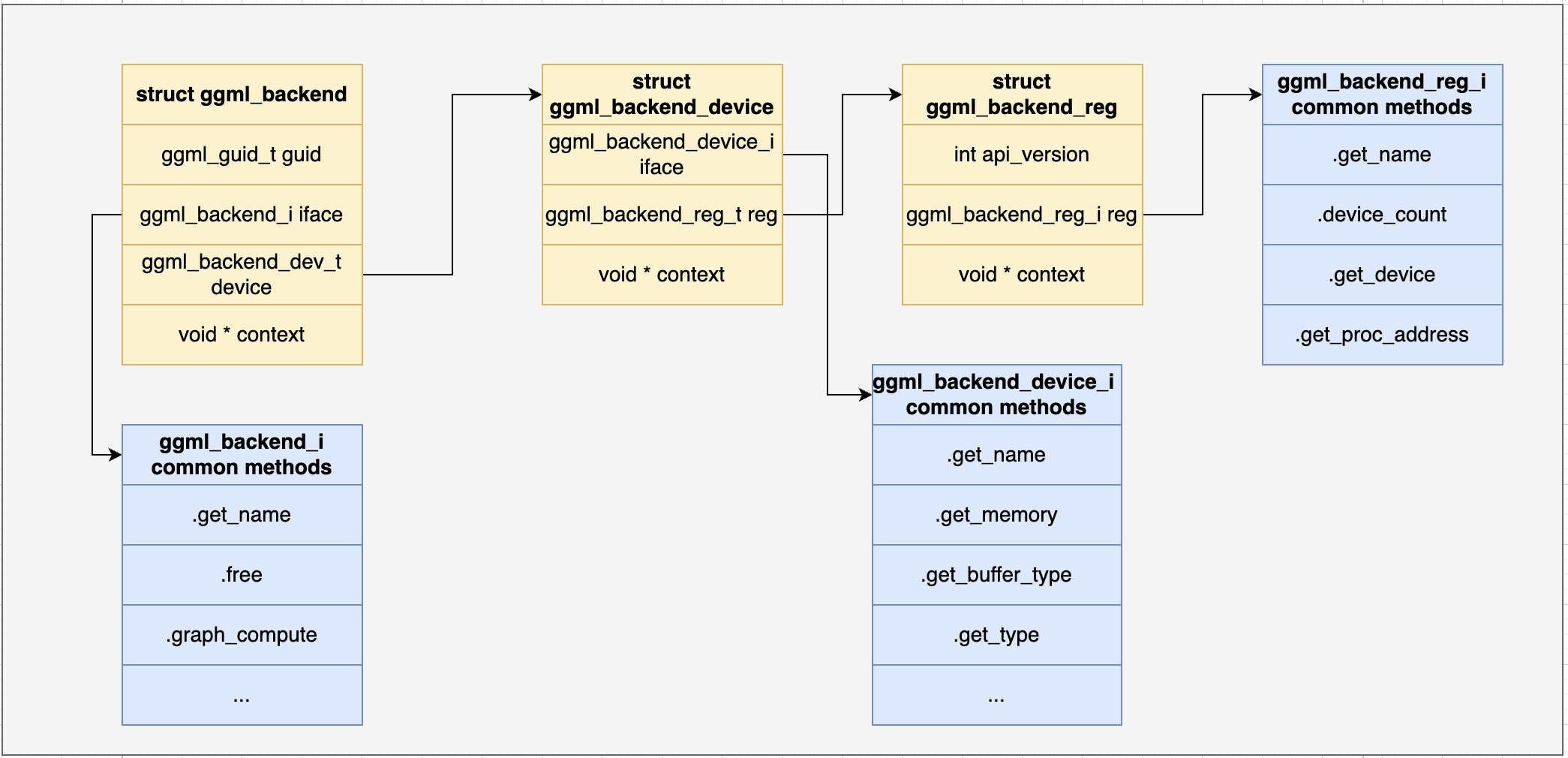
Let’s take a look at the following graph, which illustrates the common framework used by all backends in GGML.

Some key notes:

The content in any void* context is highly backend-specific and normally you don’t need to pay attention to them.
Each backend has three types of interfaces: ggml_backend_i, ggml_backend_device_i, and ggml_backend_reg_i.
GGML uses function pointers to implement polymorphism in C, a common technique in C programming. Specifically, structs like ggml_backed act as base classes, void *context contains child classes’ additional member variables, and iface defines abstract methods.

As we proceed, keep in mind that all interactions with backends happen through these three sets of interfaces. You don’t need to read through the actual backend implementation for now.

GGML Context & Tensor Creation (Similar to `simple-ctx`)

After the backend is initialized, we see a familiar pattern: creating a ggml_context. However, this time no_loc is set to true, meaning the ggml_context will only contain metadata and no longer store actual data, such as tensor weights. This is necessary because backends like CUDA won’t work if we store all parameters on the CPU. Instead, the actual parameters will be stored in backend-specific locations.

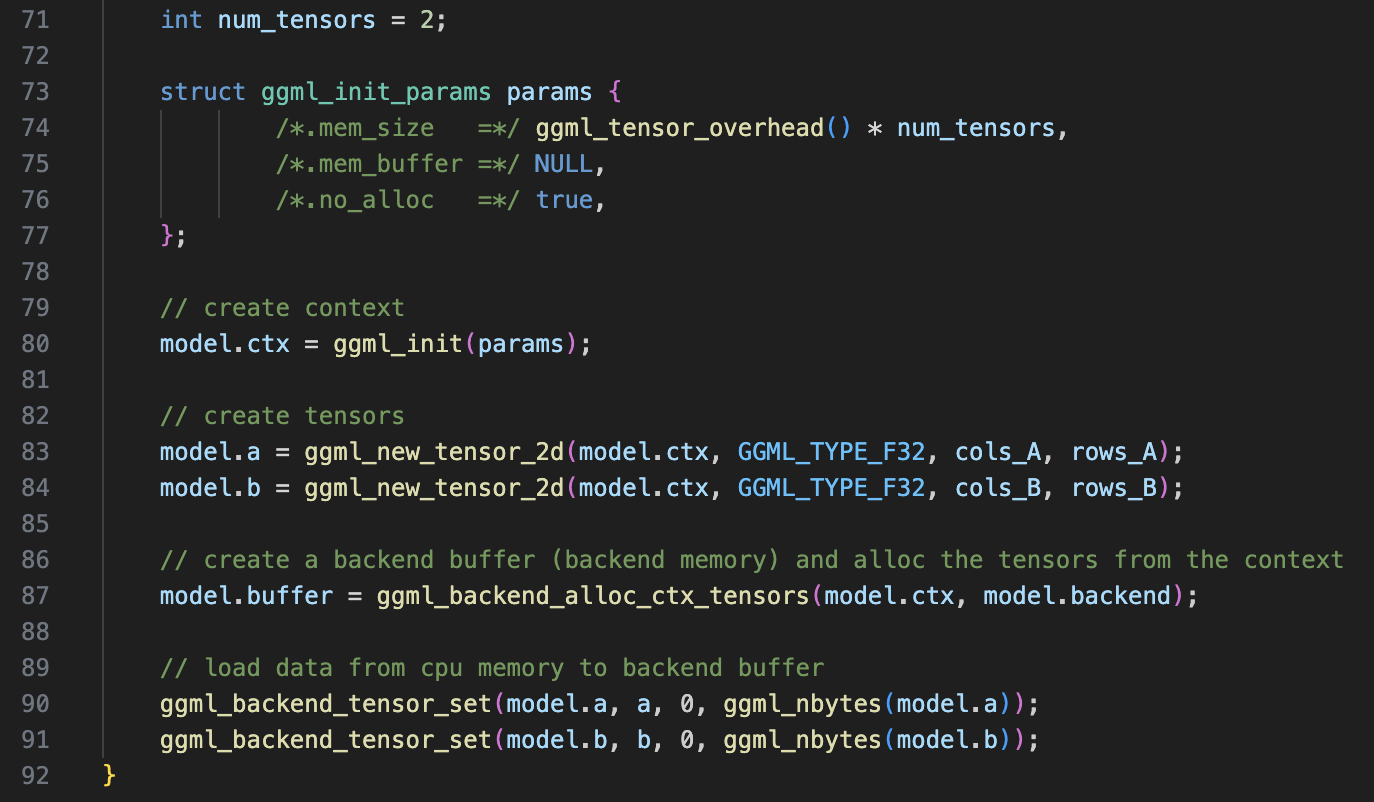
This step is achieved by two functions: ggml_backend_alloc_ctx_tensors (which allocates space for tensors in the backend) and ggml_backend_tensor_set (which loads the actual tensor data into pre-allocated space).

Before we dive into the internals of these two functions, let’s explore another class diagram for “buffers”:

Like backends, buffers can be interacted with through a set of unified interfaces (ggml_backend_buffer_type_i and ggml_backend_buffer_i).
There are both “buffer” and “buffer type”: ggml_buffer_type records metadata for the buffer, while ggml_buffer contains actual data and methods for managing the buffer.

Once you understand how buffers work, we can look into the ggml_backend_alloc_ctx_tensors function. Stepping into this function, we eventually reach ggml_backend_alloc_ctx_tensors_from_buft. Here’s what it does:

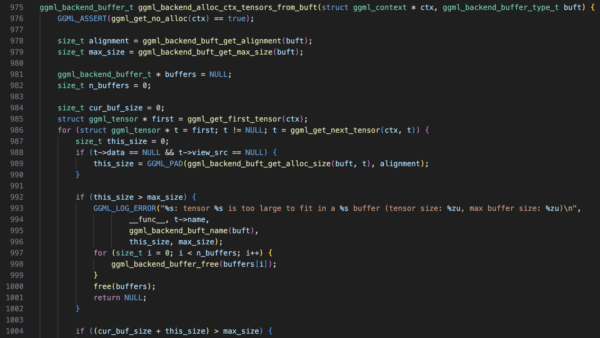
Retrieves metadata about the buffer type (alignment, max size, etc.). If you step into these functions, you’ll see that they eventually call interface methods defined in ggml_backend_buffer_type_i.
Iterates over all ggml_tensors in the ggml_context (as mentioned in the previous post, tensors are organized in a linked list).
Calls alloc_tensor_range to allocate memory in the backend’s buffer.

Now let’s take a deeper look at step 3 and examine what alloc_tensor_range does.

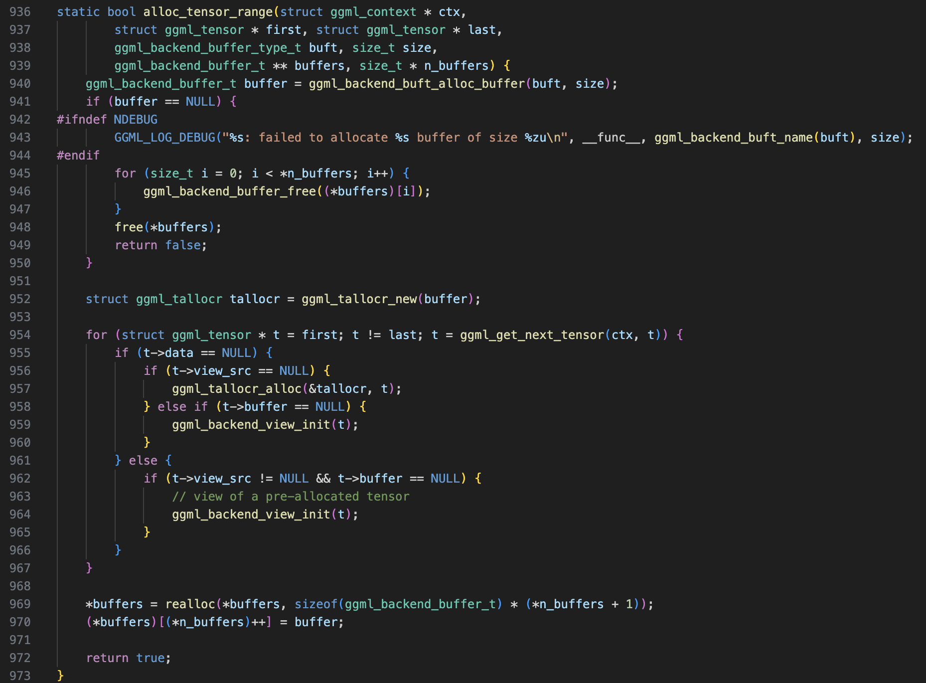
First, it constructs a tensor memory allocator, ggml_tallocr. This structure provides a convenient way to allocate memory on a buffer for tensors.

struct ggml_tallocr {
    ggml_backend_buffer_t buffer; // pointer to the buffer
    void * base; // based address in the buffer
    size_t alignment;
    size_t offset;
};

Next, it iterates over all tensors, allocating them in a continuous memory region within the buffer, and updates the ggml_tensor’s buffer and data fields to point to the corresponding location in the buffer (this happens in the ggml_backend_tensor_alloc function).

After ggml_backend_alloc_ctx_tensors returns, memory for all tensors has been allocated, but no actual data has been loaded yet. The next step is to call ggml_backend_tensor_set to load tensor data into the backend’s buffer.

Computational Graph Construction

In contrast to simple-ctx, constructing a computational graph in simple-backend is more complex since tensor memories are no longer allocated inside the ggml_context.

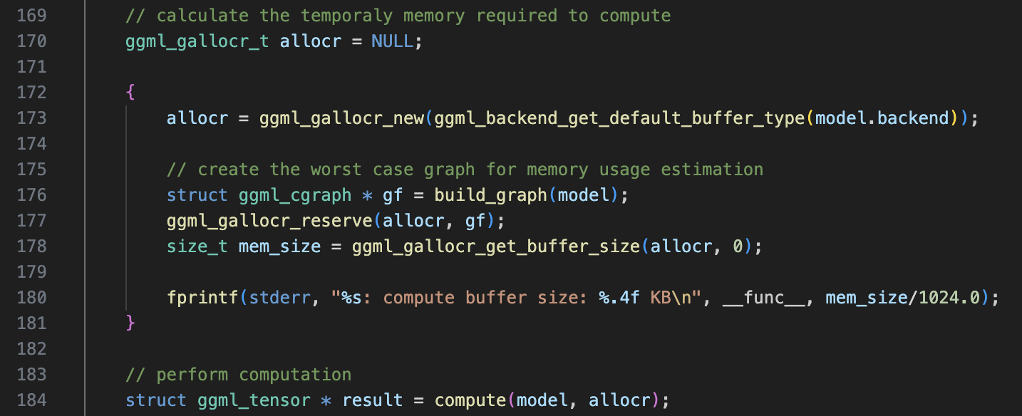
Here, GGML uses a ggml_gallocr (as the name suggests, it manages memory allocation for the computational graph) to handle memory during computation. Let’s take a look at its structure:

struct ggml_gallocr {
    ggml_backend_buffer_type_t * bufts; // [n_buffers]
    ggml_backend_buffer_t * buffers; // [n_buffers]
    struct ggml_dyn_tallocr ** buf_tallocs; // [n_buffers]
    int n_buffers;

    // Note: not the same hash set in ggml_cgraph
    struct ggml_hash_set hash_set;
    struct hash_node * hash_values; // [hash_set.size]

    struct node_alloc * node_allocs; // [n_nodes]
    int n_nodes;

    struct leaf_alloc * leaf_allocs; // [n_leafs]
    int n_leafs;
};

Although it has many fields, none are unfamiliar to us. Essentially, it consists of two parts: the first part (bufts to n_buffers) handles buffer-related fields (buffer, buffer type, and tensor allocator), while the second part (from hash_set to n_leafs) records the allocation information for ggml_tensors, such as which buffer the tensor is allocated on (hash_node.buffer_id).

Next, the graph is built using the build_graph function. Don’t confuse it with the build_graph from simple-ctx; they’re quite different.

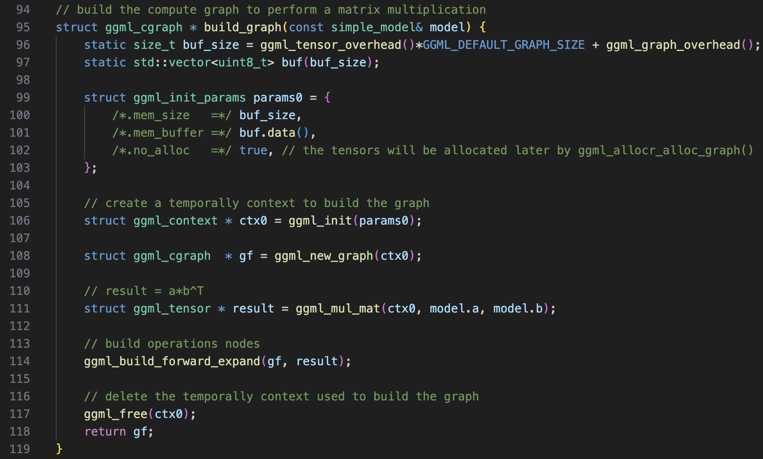
This function does the following:

Calculates the memory needed to store all ggml_tensor and ggml_cgraph.
Uses a temporary ggml_context to create the computational graph.
Creates the result tensor and stores all tensor information in the computational graph (similar to simple-ctx).
Deletes the ggml_context. Note that the memory region for ggml_context (the mem_buffer) is allocated in a static variable, so deleting the ggml_context won’t free the memory.
Returns the ggml_cgraph created.

Once the graph is created, the next step is pre-allocating memory for computation using the ggml_gallocr_reserve function.

Memory Allocation for Computation

Let’s dive into ggml_gallocr_reserve_n. The first thing it does is initialize the memory allocator’s hash table. Note that this hash table differs from the one in ggml_cgraph. In ggml_cgraph, GGML simply allocates a hash table that can represent a graph with up to GGML_DEFAULT_GRAPH_SIZE nodes. In contrast, the hash table here is more fine-grained, sized according to the actual number of nodes in the graph.

struct ggml_hash_set {
    // number of entries in the hash table
    size_t size;
    // whether or not the keys are in use i.e. set
    ggml_bitset_t * used;
    // actual tensors in the set, keys[i] is only defined if ggml_bitset_get(used, i)
    struct ggml_tensor ** keys;
};

After that, it enters the ggml_gallocr_alloc_graph_impl function, which is quite complex but contains detailed comments. You can dive into it if you’re interested, though I haven’t explored it deeply myself : )

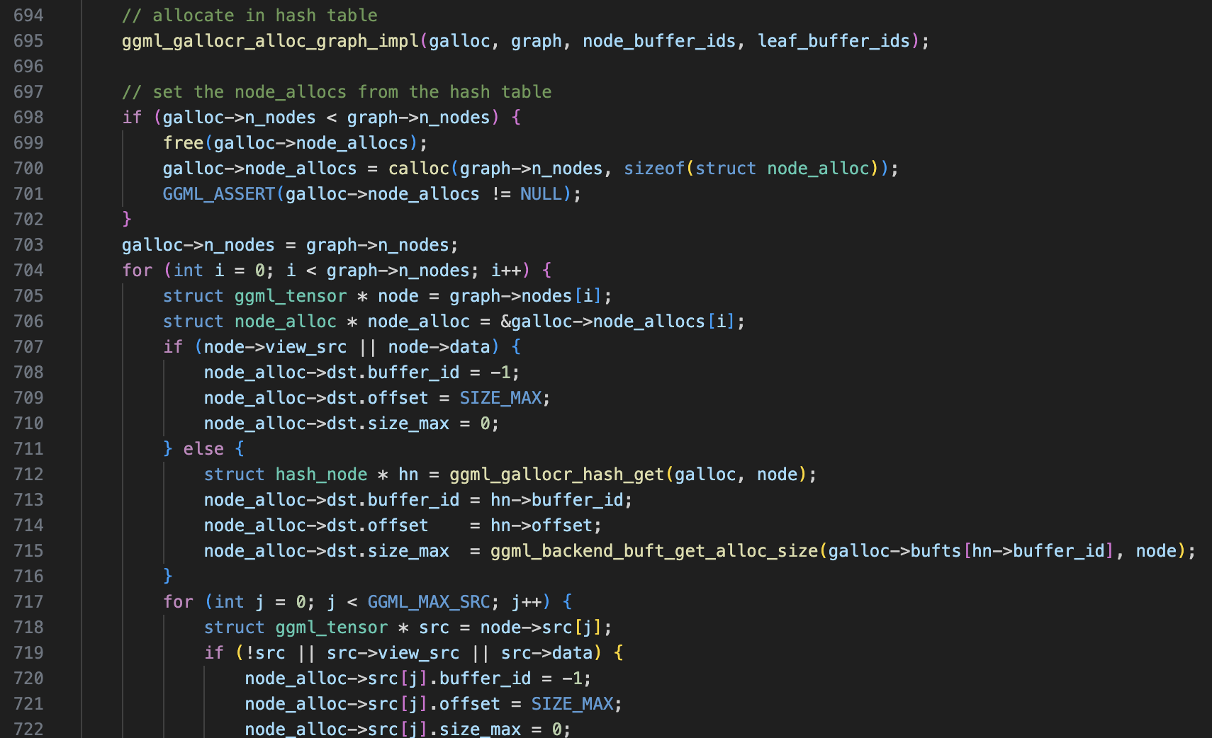
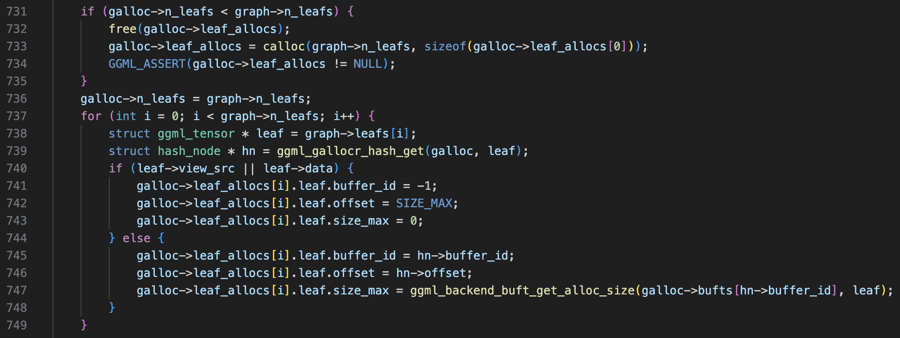
Next, it allocates ggml_galloc.node_allocs and fills in its fields. Each element in node_allocs corresponds to one tensor and records the buffer allocation information for that tensor and its source tensors. Similiar operations are applied for leaf nodes, with the only difference being that the allocator only records the leaf’s allocation information (since leaf nodes have no source tensors).

Graph Computation

Once memory allocation is complete, the final step is performing the actual computation. Let’s take a look at the ggml_backend_graph_compute function. Surprisingly (or sadly), it simply calls backend->iface.graph_compute, passing the computation task to backend-specific code. Since different backends handle this task in vastly different ways, I won’t dive into its implementation here.

TODO: Analyze the computation process of one backend.

Finally, we copy and print the result tensor, which is a straightforward operation.

Wrapping Up

In this blog, we explored how computation works in backend mode. There are some interesting observations:

All backends can be accessed through a unified set of interface methods (polymorphism in C programming).
GGML allocates memory for tensors and the computational graph in backend buffers, rather than in ggml_context.
ggml_context no longer plays a central role in GGML’s workflow.

Now, through the simple-ctx and simple-backend examples, we have a nearly comprehensive understanding of GGML’s workflow. In the next post, I’ll cover the remaining components, such as GGUF file reading using the mnist example. See you then!

Introduction#

Initializing the Backend#

GGML Backend Classes and Their Relationships#

GGML Context & Tensor Creation (Similar to simple-ctx)#

Computational Graph Construction#

Memory Allocation for Computation#

Graph Computation#

Wrapping Up#