Introduction
In the previous post, we explored how GGML, in context mode, allocates and manages memory using ggml_context and ggml_object. We walked through this mechanism in the load_model function. Now, it’s time to delve into how GGML executes actual tensor computations on top of ggml_context.
In this blog post, we’ll explore how GGML constructs and manages the data structures required to represent a computational graph. Let’s get started!
Note: This blog series is based on commit 475e012.
Constructing Computation Graph in ggml_context

Continuing from the previous post, we have completed the analysis of load_model and are now ready to step into the compute function (line 101 in simple-ctx.cpp). The first operation in this function is build_graph, where we encounter a somewhat familiar function: ggml_new_graph.
Previously, we explored the ggml_new_tensor function, which allocates and manages tensor resources using ggml_object. Similarly, ggml_new_graph follows the same approach—it creates a new node in ggml_context’s linked list and allocates a contiguous memory region within ggml_context. The key difference is that instead of storing a tensor, it manages a computation graph (we will see its structure very soon).

Stepping into ggml_new_graphuntil we reach ggml_new_graph_custom, where the first function encountered is ggml_graph_nbytes. Looks familiar?Actually we have met it before inload_model, though we skipped its details at the time. Now, with more context about how ggml works, we can dive deeper into its implementation.

The first value we see is GGML_DEFAULT_GRAPH_SIZE = 2048, a hard-coded constant that defines the maximum number of nodes and leaf tensors that can be allocated in a single ggml_cgraph. We then calculate another value, hash_size, using ggml_hash_size.
Looking at its implementation, we see that it finds the smallest prime number greater than or equal to 2 * GGML_DEFAULT_GRAPH_SIZE using binary search, which determines the size of the computational graph’s hash table. The choice of a prime number is primarily for performance consideration: GGML employs a simple open-addressing hash function with linear probing:
Key = (ggml_tensor_pointer_value / 4) % table_size
In this case, usikng a prime table size helps distribute keys more uniformly, reducing clustering and improving lookup efficiency.
Next, we compute the total memory required for various components of the computational graph:
- A
ggml_cgraphstruct to hold metadata. - 2048 pointers to
ggml_tensor, reserved for nodes. - 2048 pointers to
ggml_tensor, reserved for leaf tensors. hash_sizepointers toggml_tensor, representing hash table slots.- Pointers for gradient tensors (not enabled in our case).
- Memory reserved for the hash table mask.
A closer look at the hash table mask computation:
typedef uint32_t ggml_bitset_t;
static_assert(sizeof(ggml_bitset_t) == 4, "bitset_t constants must be updated");

// log2(4*8) = 5
#define BITSET_SHR 5

// 32 - 1 = 31 (0001 1111)
#define BITSET_MASK (sizeof(ggml_bitset_t) * 8 - 1)

// Calculates the number of ggml_bitset_t needed to store n bits
// Each bit corresponds to a hash table slot, so n is the hash table size.
// (n + BITSET_MASK) ensures rounding up when n is not a multiple of 32.
// Right shift divides the value by 32.
static size_t ggml_bitset_size(size_t n) {
    return (n + BITSET_MASK) >> BITSET_SHR;
}
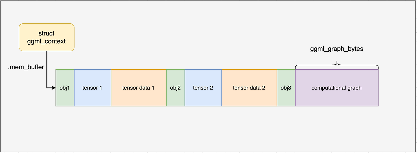
After computing the total required size, ggml_graph_nbytes returns, and we observe a familiar pattern: GGML creates a new ggml_object in the context to “hold” the computational graph, as shown below:

This includes the ggml_cgraph struct, memory for nodes and leaf tensors, hash table keys, and the hash table mask. If you recall our discussion on ggml_tensor creation from the previous blog, this process should seem quite familiar.
The next few lines initialize pointers to different regions within the allocated memory, storing them in the ggml_cgraph struct. Finally, the hash table is reset, marking all slots as unoccupied.

Filling Computational Graph with Actual Graph Information
At this point, we have successfully created a computational graph. However, this graph is still “empty”: while it has sufficient memory to hold any computation graph with nodes up to GGML_DEFAULT_GRAPH_SIZE, it does not yet contain any actual graph information. Our next step in build_graph is to construct the graph and store its information in ggml_context .

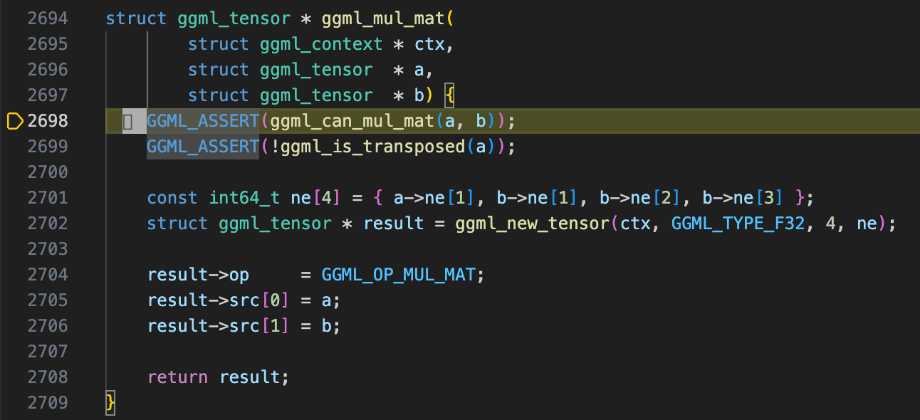
First, let’s examine ggml_mul_mat. Despite its name, this function does not perform any actual computation. Instead, GGML follows a static graph-based approach (construct the whole graph then compute, similar to TensorFlow) rather than a dynamic graph approach (like PyTorch). In ggml_mul_mat, GGML:
- Creates a new
ggml_tensorstruct to represent the result of matrix multiplication. - Computes the dimension of the output tensor.
- Stores both input tensors as its sources (child tensors store pointers to parent tensors).
- Returns the newly created
ggml_tensor.

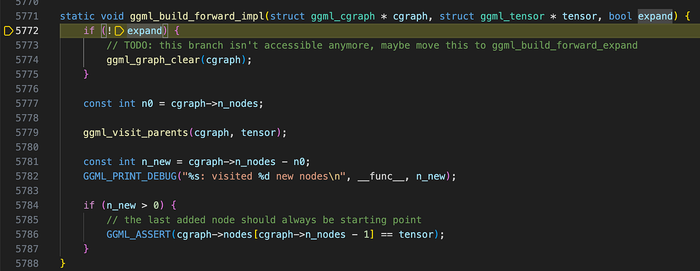
Now, we move to the final stage of computational graph construction. At this point, we have an empty graph and a result tensor, and ggml_build_forward_expand will populate the graph with the necessary computation details. This function takes two arguments: a pointer to ggml_cgraph and a result node. In this case, the node represents the result tensor of a matrix multiplication, but in more complex scenarios, it could correspond to the final output of a neural network—such as predictions from an image classifier or logits from an LLM.
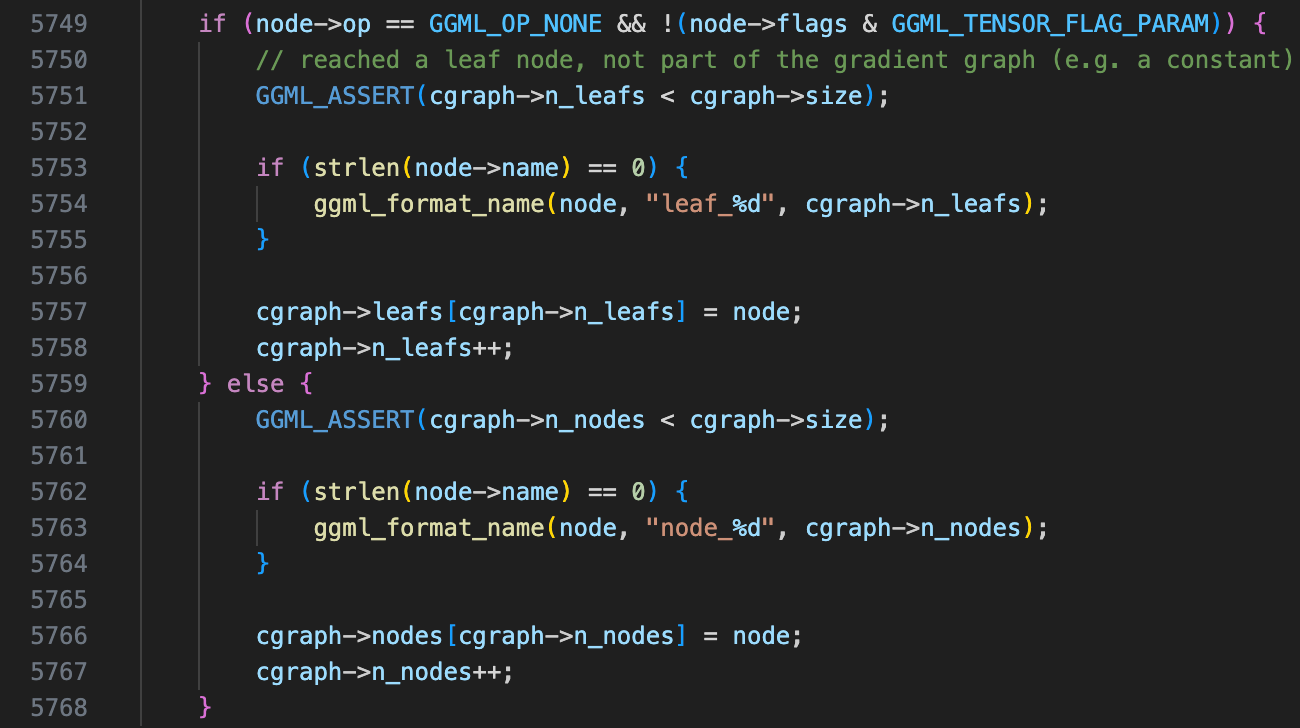
Stepping into ggml_build_forward_impl, we could see a function ggml_visit_parents, which builds the graph recursively. Its functionality can be summarized as follows:

- Check if the current tensor already exists in the hash table. If it does, stop execution and return.
- Recursively call the function on all parent tensors based on the defined evaluation order.
- After processing parent tensors, handle the current tensor:
- If it is a leaf node (i.e., a constant tensor or an input tensor not produced by an operation), store it in the graph’s leaf array.
- Otherwise, store it in the graph’s nodes array.
After all recursive calls return, a final check ensures that the last recorded node is the result tensor. This should always be the case since post-order traversal is used, meaning the input node (tensor) is inserted last.
Wrapping Up
At this stage, we have successfully built a computational graph inside ggml_context. In the next blog post, we will explore how GGML, with the aid of a computation plan (ggml_cplan), performs computation to obtain matrix multiplication results.
