Introduction

Continuing from the previous post, if you’ve followed all the steps outlined earlier, you should now be able to debug any example provided by GGML. To make the thought process as clear as possible, the first example we will analyze is simple, specifically ./examples/simple/simple-ctx.

Essentially, this example performs matrix multiplication between two hard-coded matrices purely on the CPU. It is a minimal example compared to real-world GGML applications—it involves no file loading or parsing, is hardware-agnostic, and, most importantly, all computations occur exclusively on the CPU, with all memory allocations happening in RAM. These characteristics make it an excellent candidate for demonstrating the core GGML workflow.

Note: The ‘context mode’ demonstrated in this example is no longer the best practice for using GGML. However, it remains useful for understanding GGML’s internal workflow. Later, we will explore more complex cases involving multiple hardware backends (./examples/simple/simple-backend). This blog series is based on commit 475e012.

Tips for C/C++ Source Code Reading

Here are some techniques I find useful when reading a C/C++ project’s source code for the first time. You can apply them while debugging GGML:

1. Set a breakpoint at the first line of main, then follow the execution flow step by step until the program terminates.
2. Step over functions that seem unimportant or are not directly related to the current focus (like profiling / debug printing codes).
3. Ignore assertions unless they are triggered.
4. Skip padding and alignment operations unless they are essential for understanding the code.
5. Track pointer values, calculate offsets, and sketch out a memory layout (either mentally or on paper).

Tip #5 is particularly useful when analyzing GGML, as you’ll soon discover in this post. No worries if you’re not familiar with drawing memory layout diagrams — I’ve included some in this post : )

The First ggml_context

Let’s begin with the simple-ctx test case. Set a breakpoint at the first line of main and start following the execution flow. Skip ggml_time_init (per Tip #2: ignore unimportant functions), and step into load_model, where you’ll encounter a seemingly intricate computation for ctx_size. We’ll defer understanding these calculations until we have more context on GGML’s internals.

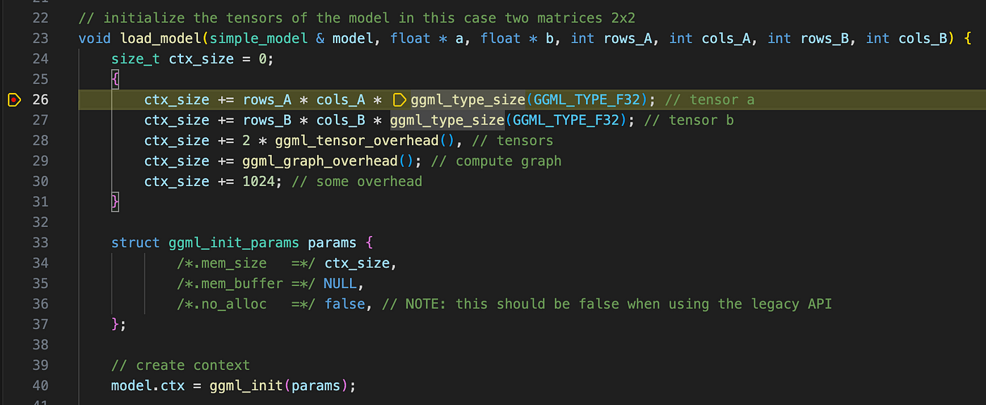
Next, we reach one of the most important functions in GGML: ggml_init().

Understanding ggml_init()

The ggml_init() function takes three arguments packed in a struct:

• ctx_size (calculated earlier)
• A null pointer
• A flag set to false (we’ll understand its purpose later)

Stepping into the function, the first section is straightforward — it initializes a lookup table for fast FP32-to-FP16 type conversion if this function is called for the first time. Moving past that, we see that a new ggml_context struct is allocated on the heap.

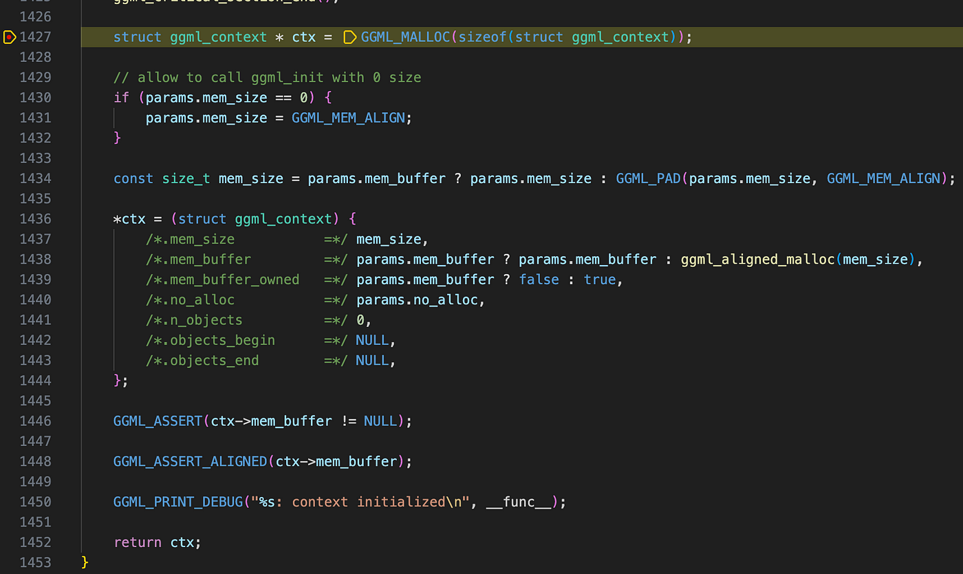
The next few lines may look confusing initially, we can focus on three key struct members:

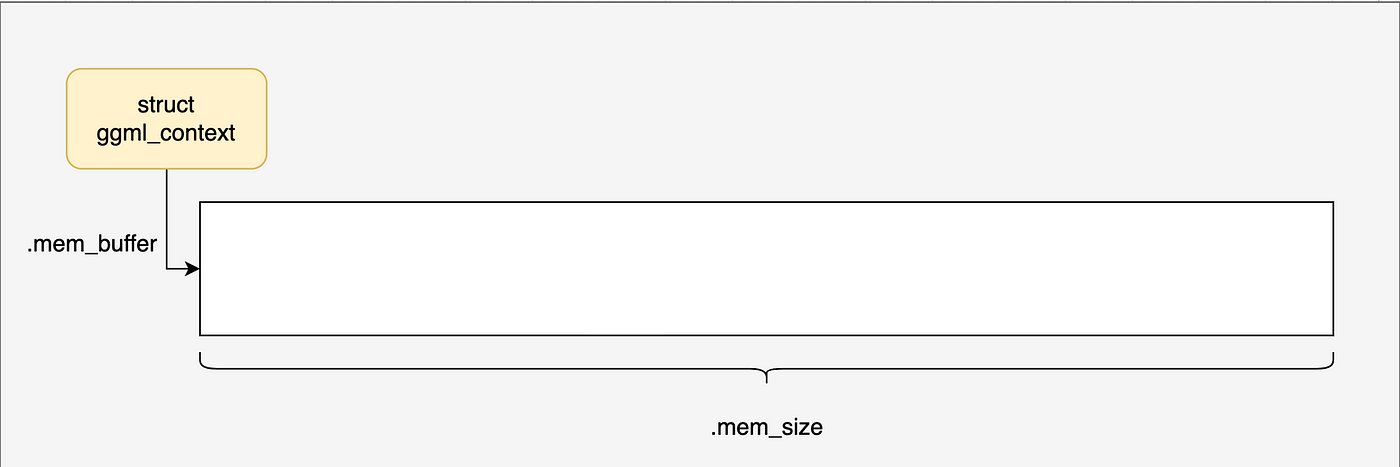
• **mem_buffer**: A pointer to a memory region on the heap. If the mem_buffer member of the params argument passed to ggml_init is not nullptr, it means we want to use an existing allocated memory block for ggml_context. Otherwise (mem_buffer == nullptr), a new memory region is allocated.
• **mem_size**: The size (in bytes) of the memory region pointed to by mem_buffer.
• **mem_buffer_owned**: Indicates whether the ggml_context is using its own memory allocation.

At this stage, the memory layout of our ggml_context is structured as follows:

You might wonder: if **ggml_context** only holds a piece of memory, what is its actual purpose? Let’s explore this further.

Tensor Dimension Representation in GGML

Stepping out of ggml_init, we now reach two calls to ggml_new_tensor_2d. Step into the first function call recursively until you reach ggml_new_tensor_impl. The view_src related lines can be ignored for now, as it primarily handles the tensor views, which does not exist in our case.

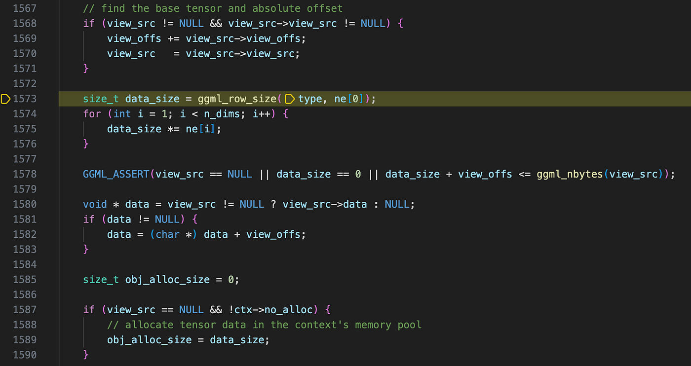
To grasp ggml_row_size, we must first understand how GGML represents tensor dimensions. Unlike frameworks such as PyTorch, where dimensions are listed from outermost to innermost (left to right), GGML uses a 4-element array (yes, ggml only supports up to 4-d tensors, as it is sufficient for LLMs)ggml_tensor.newhere the innermost dimension appears on the left. This is the opposite of PyTorch’s representation, for example, a PyTorch tensor with shape [20, 10, 32, 128] will be represented as ggml_tensor.ne = {128, 32, 10, 20} in ggml.

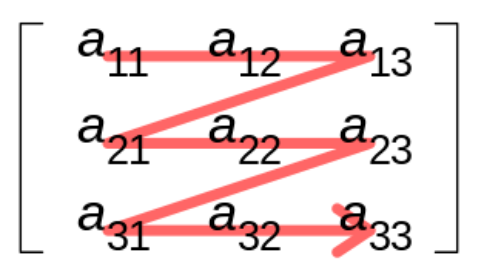
Note: here the innermost dimension refers to the one where memory is contiguous. For instance, for row-major storage in C/C++, the column dimension is the innermost dimension as shown below:

Now, take a look at ggml_nbytes(). Since our matrix uses float32 data types, this function simply returns the number of bytes required for a single row (sizeof(float) * number of elements in a row). If quantization were applied, this calculation would be more complex—but we’ll delve into that in future posts. Similarly, data_size represents the total size (in bytes) of current tensor.

Let’s continue. A critical part of GGML’s memory management lies in this condition:

In our case, since view_src is nullptrand no_alloc is set to false, the following line is executed:

obj_alloc_size = data_size;

From its name, we can infer that this value represents the amount of memory needed to allocate for storing the tensor. But where is this value used? The answer lies in ggml_new_object.

Understanding ggml_new_object()

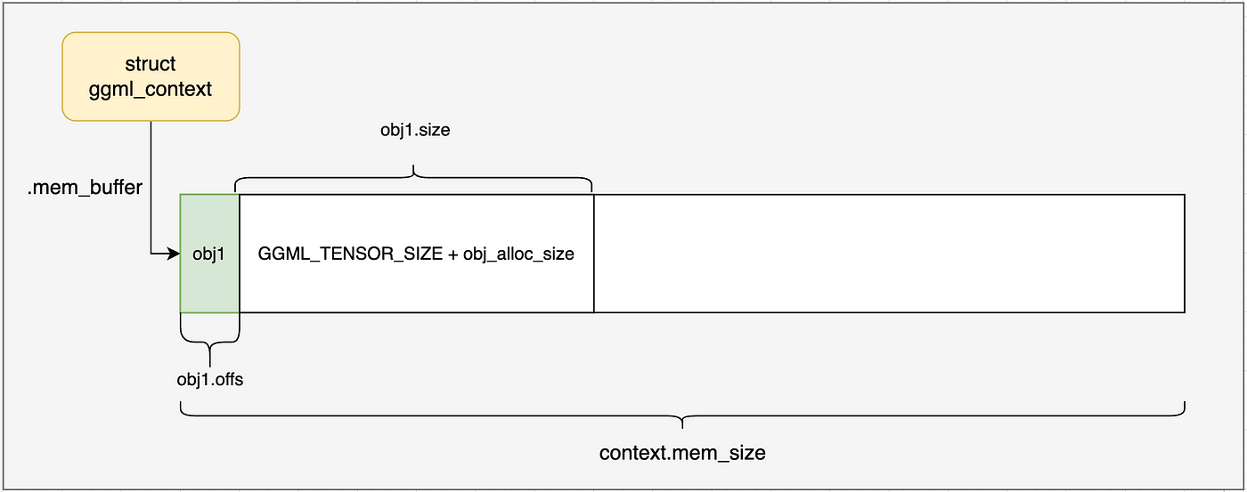
Stepping into ggml_new_object(), the implementation here may be challenging to understand if you read it sequentially, you can break it down and understand it in the following order (you can also scroll down to view the memory layout graph for this section first):

1. Take a look at the definition of ggml_object, each ggml_object has a next pointer pointing to another ggml_object . Based on its type and naming, apparentlyggml_objects could form a linked list, with each ggml_object being a list node.
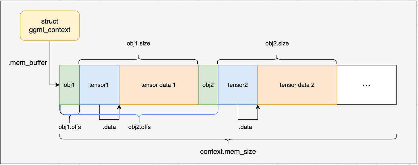
2. Initially, ggml_context.objects_begin and ggml_context.objects_end are nullptr. Each time ggml_new_object() is called, a new ggml_object is added to the end of the linked list, updating the next field of the previous ggml_object and ggml_context.objects_end to point to the new ggml_object.
3. What is the purpose of ggml_object? Linked lists are commonly used for O(n) time resource lookups, and GGML is no exception. Each ggml_object implicitly manages a specific resource—it could be a tensor, a computation graph, or a work buffer (for now, we’ll focus on tensors).
4. For a ggml_object that holds a ggml_tensor, how much memory does it require within the ggml_context? It is:

• GGML_OBJECT_SIZE (sizeof(struct ggml_object)) + GGML_TENSOR_SIZE (sizeof(struct ggml_tensor))+ obj_alloc_size
• Now we can draw the memory layout when the first call to ggml_new_object returns (note that no new memory block is allocated here, everything happens in ggml_context.mem_buffer):

ggml_tensor Definition

Now that we have a ggml_object and understand that it “holds” the ggml_tensor we need to place inside the ggml_context, the next question is—how exactly does this happen?

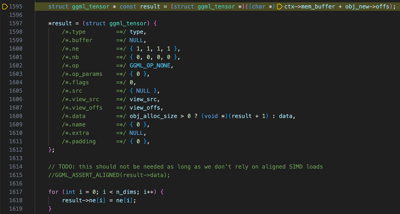
Recalling from the previous section, it is not hard to tell that ggml_tensor *const result points one byte past the ggml_object. This is precisely where the ggml_tensor should be stored. We treat this region in memory as a ggml_tensor struct using pointer type casting, then initialize it with default parameters. Here is the memory layout graph at this point:

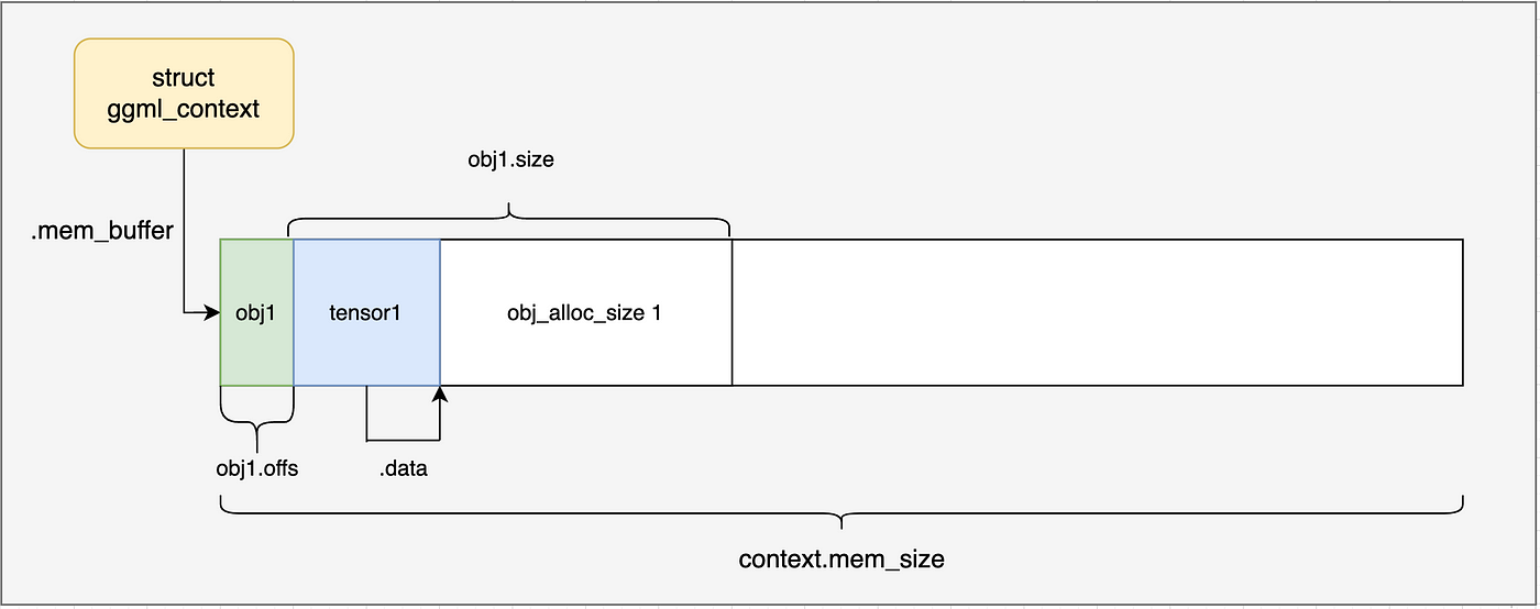
For now, we’ll focus on three key fields of ggml_tensor:

• data: A pointer to the start address of the actual tensor data. In this case, it points to one byte past the ggml_tensor struct itself.
• ne: An array of size 4 that represents the number of elements in each dimension. We’ve already discussed its meaning—it defines the shape of the tensor, in this case it is [2, 4, 1, 1] .
• nb: Another array of size 4. Similar to ne,but instead of storing number of elements like ne, it holds the number of bytes for each dimension. Since no quantization or alignment is applied in this case, nb[i] is simply calculated as:

nb[0] = sizeof(float);
nb[1] = nb[0] * ne[0];
nb[2] = nb[1] * ne[1];
nb[3] = nb[2] * ne[2];

Now that we understand what happens inside ggml_new_tensor_2d, let’s examine the memory layout after two consecutive calls to it (after line 44 in simple-ctx.cpp):

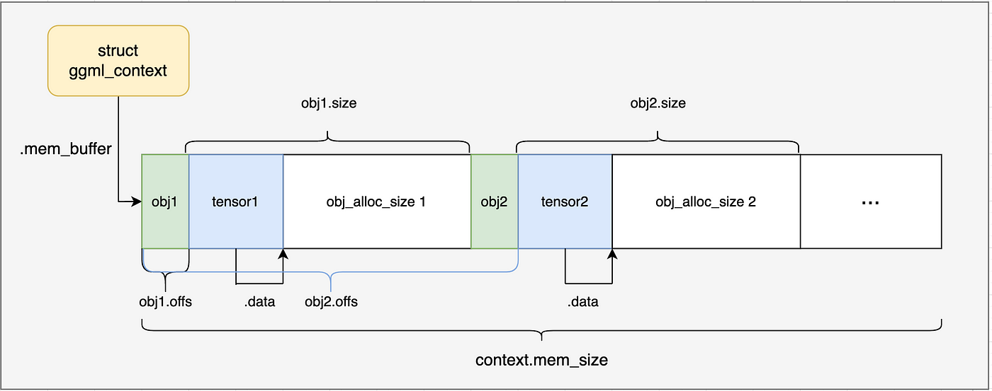
Finally, we copy the tensor data into ggml_context through memcpy, marking the completion of load_model.

Note: In this case, the tensor data is defined directly within the source code, so there is no need for GGUF file loading. However, in more complex examples, such as ./examples/mnist, this step becomes essential.

Wrapping Up

In this post, we examined how GGML manages memory in context mode, including:

• How ggml_context handles memory allocation.
• The structure and functionality of ggml_object.
• The way ggml_tensor is represented in memory.

In the next post, we’ll explore how GGML constructs a static computation graph and executes computations on it. Stay tuned!